TomoTree Web Application — User Guide
Overview
TomoTree GUI is a web application for acoustic tomography of trees. It processes travel-time or sound-speed measurements between sensor nodes placed around a tree cross-section and reconstructs a 2D tomogram that shows the internal condition of the wood.
The application can be used by arborists and researchers to identify areas of decay, cavities, or mechanical weakening inside a living tree without invasive methods.
Login and Registration
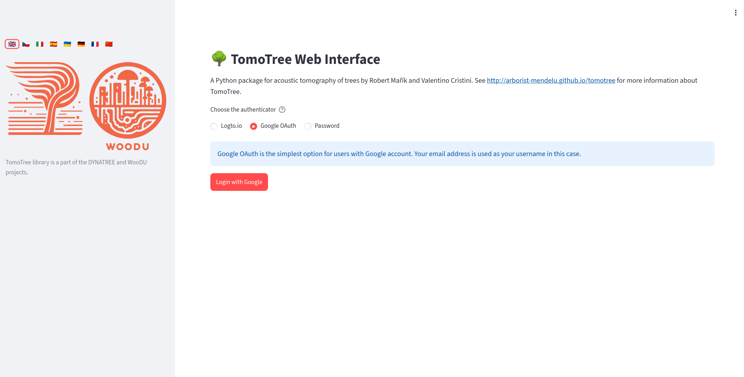
Login screen allows password access and also access via social accounts (if configured by the administrator).
The login page is configured by the site administrator. There are the following options:
local account, with possible new account registration,
login via social accounts (Google or accounts registered in Logto.io service)
If the GUI runs on a localhost, it is typically fine to run the application without login protection and without user management. In this case, the login page is skipped and the user is automatically logged in as a default user.
Home Screen and Data Source
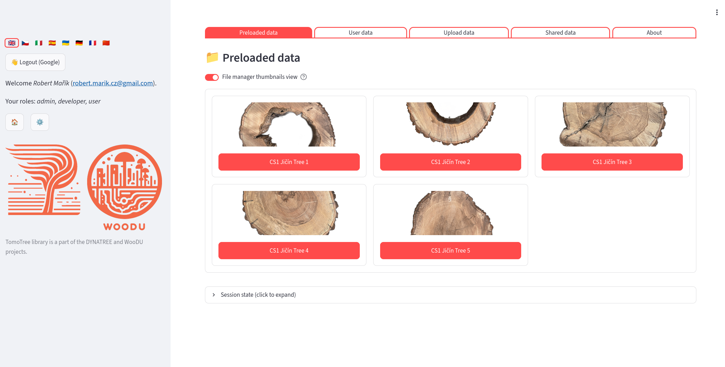
Home screen shows available datasets. You may upload your own data, load preloadeed data or load data shared by other users.
After login you choose which dataset to work with.
Preloaded Data
A gallery of datasets prepared by the administrator. Each dataset is shown as a thumbnail image with a title. Click any dataset to open it in read-only mode.
User Data
Your personal storage directory. You have read-write access. Every directory here is one dataset (typically one tree or one measurement). You can:
Create a new dataset directory (➕ New measurement): enter the name, optionally keywords and files (sorted into the folders of the dataset by type); 📂 Create and open opens it at once.
Open a dataset (✅), manage its files (🗂️), download it as ZIP (📦), rename it, edit its keywords, or delete it (🗑️).
Filter datasets by name or keywords and sort them by name or size.
See Where Your Data Are Stored for the layout of files inside a dataset.
Upload Temporary Data
Use this tab to load data that is not yet on the server. The uploaded files (or an extracted ZIP archive) are stored in a temporary directory that does not count towards your storage quota and is not kept permanently. If you later decide to keep the data, use the button in the sidebar to copy them into your user directory as a new dataset.
Where Your Data Are Stored
Storage areas
Area |
Access |
Where on the server |
Counts to quota |
|---|---|---|---|
Preloaded data |
read-only |
|
no |
User data |
read-write (owner) |
|
yes |
Shared data |
read-only |
|
owner’s quota |
Temporary upload |
read-write |
a temporary directory ( |
no |
The directory names are the defaults; the administrator can change them in config/config.yaml (keys dirname, userdir, shareddir). Because a shared dataset is only a link, any change made by the owner is immediately visible to everybody the dataset is shared with.
Layout of a dataset
The name of the dataset directory is chosen by the user. Inside the dataset, every kind of data has its own fixed subdirectory, so the application finds the files automatically:
streamlit_user/
└── <username>/
    ├── favorites.json          # quick-access favourites of the user
    └── <dataset>/              # e.g. linden_arboretum
        ├── keywords.txt        # keywords used for filtering datasets
        ├── thumbnail.png       # optional preview image in the dataset list
        ├── config.yaml         # settings and imported data of the whole dataset
        ├── tomogram/           # nodes*.csv, distances*.csv,
        │                       # speeds*.csv, velocities*.csv, times*.csv,
        │                       # tomograph files *.f3d, *.pit, *.abt, *.mp4
        ├── backgrounds/        # photos of the cross-section (*.png, *.jpg) for Postprocessing → Background;
        │                       # without this folder the images from photos/ are offered
        ├── resistograph/       # resistograph curves (*.dpa), one file per drilling path
        ├── scans/              # 3D scans: *.obj + *.mtl + textures, *.glb, *.gltf (flat, no subfolders)
        ├── photos/             # photos for Photo assessment and saved tracings (<photo>.tracing.json)
        └── states/             # saved application states (*.state, *.state.desc.txt, autoload.state)
Kind of data |
Subdirectory |
Accepted file types |
|---|---|---|
Tomogram (geometry, measurements) |
|
csv, f3d, pit, abt, mp4 |
Background photos |
|
png, jpg, jpeg |
Resistograph |
|
dpa |
3D scans |
|
obj, mtl, glb, gltf, png, jpg, jpeg |
Photos for photo assessment |
|
png, jpg, jpeg, json |
Saved states |
|
state, txt |
keywords.txt and thumbnail.png stay in the dataset root.
Uploading files
Pages that need data files offer a 📤 Upload … button: Background, Scan tools and Photo assessment always, the tomogram and resistograph pages when no data are found. A tomogram page without sensor positions or travel times (e.g. an empty dataset) offers ⚙️ Configuration editor next to 📁 Upload tomogram files, so the data can also be typed in or pasted from a spreadsheet. The button opens a file manager already pointed to the right subdirectory and accepting only the file types listed above. The subdirectory is created on the first upload. The whole dataset can be browsed with the file manager on the User data page (🗂️) or, with an open dataset, with the 📂 File manager button. Uploads are checked against your storage quota. In read-only datasets (preloaded or shared data) the file manager only allows browsing and downloading.
Files produced by the application are stored in the dataset as well: saved states go to states/, photo tracings are saved next to the photo in photos/, and reconstructed or converted scans go to scans/.
Tomograph files
A measurement can be opened directly from the project file of the tomograph: Fakopp ArborSonic 3D (*.f3d), PiCUS (*.pit) or Arbotom (*.abt). If the dataset has no config.yaml and the tomogram/ folder has no nodes.csv, the application imports the tomograph file into config.yaml in the dataset root when the dataset is opened (sensor positions in cm, travel times in µs); the file is registered as a data source. If the folder contains several tomograph files, choose the one to open and click Open this measurement.
All devices are processed the same way: the repeated taps of one direction are combined by the mean of the taps within 20 % of their median; a direction without consistent taps gets no time and only the reverse ray of the pair is used. Pairs with fewer than 3 valid taps, valid taps scattering more than 5 % and pairs whose two directions differ by more than 20 % are reported as comments in config.yaml and in the file preview of the file manager. Nothing is excluded automatically; suspicious pairs can be reviewed in Select Rays.
The generated config.yaml also records the device (device) and its sensor numbering direction viewed from above (sensor_direction: anticlockwise for PiCUS and ArborSonic, clockwise for Arbotom), which the 3D scan pages use as the default numbering.
Older datasets (all files in the root)
Datasets created before the subdirectories were introduced have all files directly in the dataset root. They keep working without any change:
Reading: the application uses the subdirectory if it exists, otherwise the dataset root.
Writing: new files go to the subdirectory if it exists. If it does not exist but files of the same kind already lie in the root, new files are written to the root as well, so that the old files are not hidden.
When the file manager finds such files in the root, it offers a button 📁 Move N file(s) to <subdirectory>/. The move never overwrites a file that already exists in the subdirectory. Note that once a subdirectory exists, files of that kind left in the root are ignored.
Other data kept on the server
The session is saved automatically on the server (in
streamlit_session/, outside the datasets), so that your settings survive a page reload. This is independent of the explicit Save state files stored instates/.Each user has a storage limit (100 MB by default, the administrator can change it per user). The current usage is shown in the sidebar and on the User data page.
Tomography Reconstruction
Reconstruction Methods
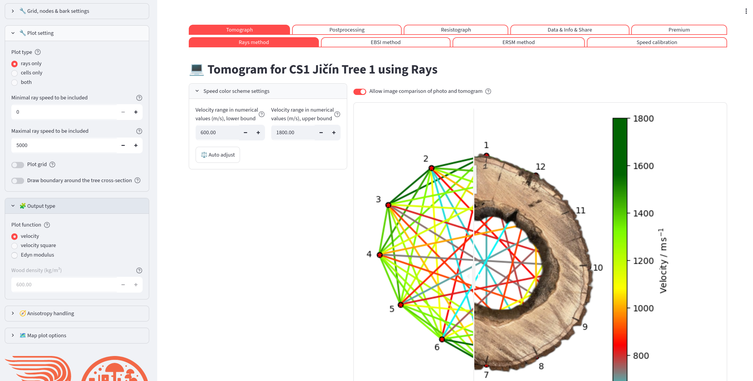
The first step in the reconstruction workflow is typically to explore the raw measurement rays. If the photo of the cross-section is available, you can superpose both images.
Reconstruction controls are available in the sidebar.
Controls (left column):
Node selector — deselect any node to exclude all rays connected to it.
nx / ny — number of grid cells in the horizontal and vertical directions.
Bark thickness — outer bark layer as a percentage of the cross-section radius.
Boundary is spline — switches between a polygonal and a smooth spline boundary through the sensors. Disabled when the boundary comes from a 3D scan (“Using the imported scan polygon as the stem boundary.”).
Coordinates alignment — origin of the coordinate axes.
Speed color range — set the minimum/maximum speed for the color scale. Click Auto adjust to reset to the 10th/90th percentile of the data.
Outputs (right column):
A color-mapped plot of all rays.
The estimated pith position (tree center) in cm.
Optional draggable image-comparison slider if a background photo is configured.
Statistics (below the plot):
Interactive ECDF and histogram of ray speeds.
Descriptive statistics table.
Ray time-of-flight comparison table and histogram.
Reconstruction Methods
The user typically chooses one of the following combinations of reconstruction method and visualization
Rays method and rays plot
EBSI method and cells plot
ERSM method and either (segmented) rays or cells plot
Rays method is the fastest preview option. No advanced reconstruction is performed — the raw measurement rays are drawn on the grid and colored by their measured speed. Use this to check node placement and spot obvious data problems before running a full reconstruction. In most cases the rays visualization is suitable for the Rays method. For distribution of the speed in the cross-section use the advanced reconstruction methods (EBSI, ERSM, SIRT or FBP). With “Rays: Ray width” in “Rays method parameters” above 0 (fat rays, e.g. 12 %), every cell gets the weighted mean speed of the rays near it, which gives a smooth preview of the whole cross-section.
The page “Tomograph → Compare methods” shows the tomograms of all five methods side by side, computed with the same settings: the settings shared by all methods (grid, anisotropy, boundary, bark, sensors, disabled rays, plot options) and, for a setting of one method only (e.g. the FBP damping), its last choice on the method page or the default. One color scale for all methods (or one per method), a summary table with the sound wood velocity, percentiles and the misfit of the measured times, and the “Reproduce in Jupyter” code (analysis.reconstruct, analysis.common_color_limits, analysis.time_misfit).
Badges above the tomogram show the settings of the computed tomogram: the method options, the anisotropy correction (orange when on), post-processing (rescaled speeds, back projection correction) and data selection (disabled rays, subset of sensors, bark).
Reading the colours
By default the colour scale is set in percent of the sound wood velocity (“Velocity scale” → “percentage of reference value”, reference “sound wood velocity”, 50–100 %). The colours then mean the same in every tree and a sound tree stays green. The scale “percentile” stretches the colours over the velocities of the tomogram, so even a sound tree shows red cells; use it only to see the details of one tomogram. The colorbar follows the velocity scale: with the percentage of a reference value it shows % of the reference (ticks at round percentages), and a green badge above the tomogram tells what 100 % is (e.g. “100 % is sound wood velocity: 1629 m/s”); with the percentile or numerical scale it shows m/s.
What the colours tell, and what they do not:
A slow region means weakened wood or a cavity, and its position and size are reliable. All methods agree on them well.
The velocity inside the defect is only an upper estimate. The device records the first arrival of the stress wave, and the wave goes around a slow region through the sound wood. For a stem of 60 cm with a defect of 20 cm and sound wood of 1500 m/s, every defect slower than about 1280 m/s gives exactly the same times of flight: an air cavity, decay of 500 m/s and decay of 1200 m/s cannot be told apart, by any reconstruction method. The tomogram therefore shows such a defect at 85–95 % of the sound wood velocity instead of its real value. Do not read “60 %” as “less decayed than 40 %”; read it as “here is a defect”.
Smaller defects (below about 8 cm across with 12 sensors) are blurred and look less slow than larger ones.
Details and the numbers: the analysis of the FBP method, chapter 27 (fbp_report.md, in Czech), and the tutorial demo/demo_03_colour_scale.py.
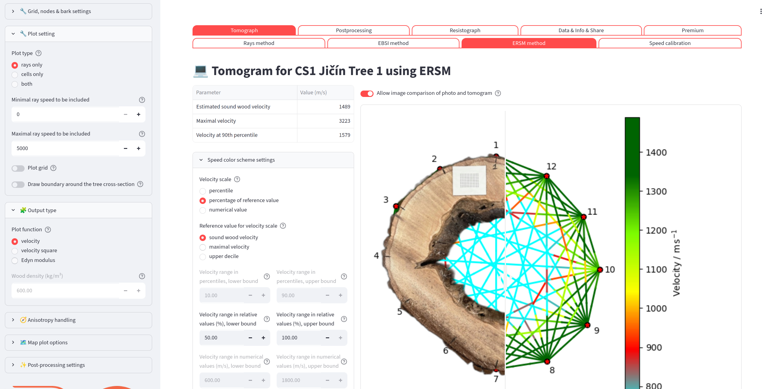
The most advanced reconstruction method in TomoTree is ERSM method. It does not utilize uniform speed along the whole ray and thus sound propagation is more realistic.
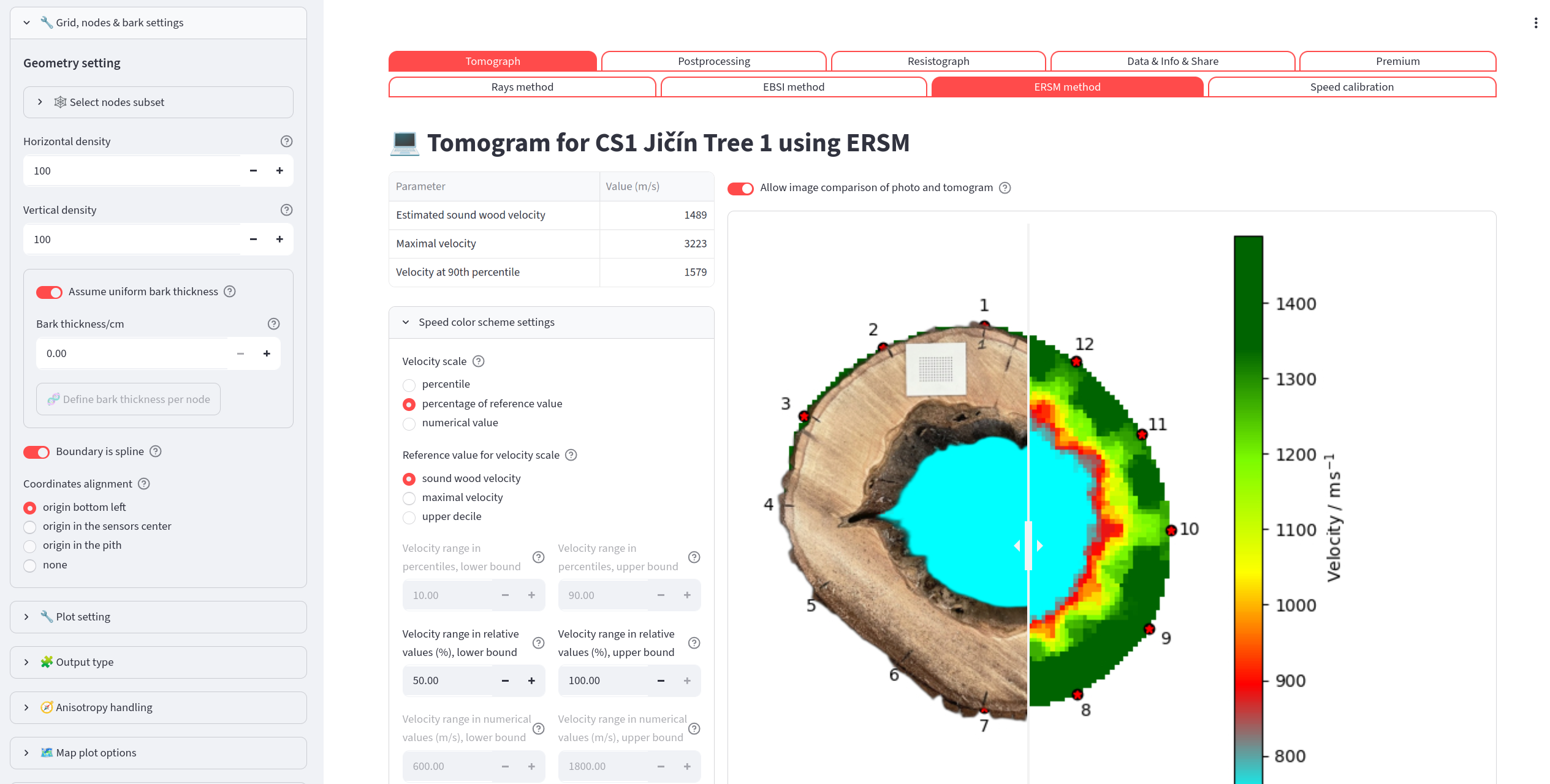
ERSM method with cell plot.
Select Rays
Tomogram pages (Rays, EBSI, ERSM) → Geometry setting → ✂️ Select rays
A dialog for leaving individual rays out of the reconstruction. Click a ray in the plot of the sensors to disable it or to enable it again; Enable all clears the selection. Disabling a ray leaves out both directions of the sensor pair. The number of disabled rays is shown under the button, and the list is part of the settings saved by 💾 Save to file (key disabled_rays in config.yaml) and of the Jupyter snippet.
Two automatic suggestions add rays to the selection; they never run by themselves:
Rays leaving the stem outline — a straight ray that crosses air cannot be the real wave path, so its velocity is underestimated and it can create false low-velocity zones near concave parts of the stem. A ray is selected when the part of its path outside the outline (green line: the imported scan outline, or the spline/polygon through the sensors) is longer than the Tolerance (cm) (default 1 cm; the equivalent percentage of the stem diameter is shown). Disable rays leaving the outline (N) adds them.
Rays measured differently in the two directions — sensor pairs whose times (or speeds) i→j and j→i differ by more than Allowed difference (%) (default 20 %) of their mean. Sensors that occur in many such pairs are named; check their coupling before disabling single rays. Disable rays with different directions (N) adds them. A difference may come from the measurement or from the wood, so look at the pairs before disabling them.
Speed Calibration
Menu: Tomograph → Speed calibration
Speed calibration is a tool for estimating the speed of sound in healthy (sound) wood from the rays that travel along the outer ring of the cross-section (tangential rays).
Workflow:
The app automatically identifies tangential rays and lists them in a pills widget labeled
<node A>–<node B>.Deselect any ray that you believe passes through degraded wood.
Optionally choose the averaging method: Mean or Median.
The estimated sound-wood speed is shown in a highlighted box and stored for use in binary thresholding and color-scale percentage mode.
Tangential rays disabled in ✂️ Select rays are not offered and not used; the page lists them.
The tomogram plot highlights (in black) the grid cells that contribute to the selected tangential rays.
Postprocessing
Binary Tomo
Menu: Postprocessing → Binary Tomo
Applies a velocity threshold to classify each grid cell as sound wood (above the threshold) or degraded wood (below it).
Controls:
Threshold source — choose between:
From color scale position — a slider sets the threshold as a percentage of the current color-scale range.
Explicit value — enter the threshold directly as m/s, as a percentage of the reference speed, or as a percentile rank.
Neutral axis — draw a red dashed line through the sound-wood region at a chosen angle.
Center of gravity — plot the geometric center of all cells (blue) and the center of sound wood (red).
Measure wall thickness — show green wall-segment indicators on the tomogram.
Binary mask background — if a background photo is registered, choose to show it under the binary mask instead of the color tomogram.
Outputs:
A draggable comparison slider between the original tomogram and the binary mask.
A moment of inertia and section modulus as functions of the angle from -90° to +90°. The charts take into account both full cross-section and sound-wood-only areas.
A second moment of area table.
Wall-thickness measurements (when enabled).
Center-of-gravity coordinates in cm.
Photo Assessment
Menu: Postprocessing → Photo assessment
Evaluates the cross-section from a photograph instead of the tomogram. The photos are stored in the photos/ subdirectory of the dataset; upload them with 📤 Upload or manage photos.
Workflow:
Select the photo in the Cross-section photograph box.
In the editor, draw the outer boundary of the cross-section as a polygon and further polygons for the areas to exclude (decay, cavities). Draw line 1 with a known real length to set the scale; optionally mark the position of sensor 1 to orient the photo.
Enter the real length of line 1 and its units, choose which polygon is the outer boundary, optionally mirror or rotate the geometry.
The page shows the full and sound-wood cross-section, their centroids, and the moment of inertia and section modulus as functions of the neutral-axis angle. The results can be downloaded as CSV.
Wall thicknesses from the photo: in the editor group Sensors, click Mark sensors and click the sensor positions in order (sensor 1, 2, 3 …); Remove last and Clear sensors correct the marking. The sensors are placed on the nearest point of the outer outline. With at least three sensors, switch on Estimate wall thicknesses from photo: the walls are measured as in Binary Tomo, on lines from the midpoint of neighbouring sensors to the centroid of the polygon of all marked sensors; the wall is the first stretch of traced sound wood along each line. Number of sensors for wall measurements (default: all marked sensors) selects fewer sensors around the stem. The lines are drawn on the photo and listed in a table. The marked sensors are saved with the tracing and are also used to place the photo on the 3D scan (see 3D Scans).
Click 💾 Save photo tracing to store the drawing as <photo>.tracing.json next to the photo. The saved tracing is loaded automatically when the photo is selected again; Reopen saved tracing reloads it. The tracing can also be downloaded as JSON.
Area Selection Tool
Menu: Postprocessing → Area selection tool
Divides the tomogram into user-defined velocity intervals and measures the cross-sectional area that falls in each interval. Similar to discrete color mapping, but with the ability to define custom intervals.
Tomogram Measurement Tool
Menu: Postprocessing → Tomogram measurement tool
Lets you interactively click or drag on the tomogram image to record coordinates and distances in real-world units.
Workflow:
Click on the image to record a point (shown in blue).
Drag across the image to place a segment — both endpoints and the Euclidean distance are recorded.
All measurements are accumulated in a table and labeled sequentially on the image.
Adjust the scale factor slider to convert output units if needed.
Click Clear all measurements to start over.
Calibration mode: Before measuring, you can calibrate by mapping two pixel positions on the image to known physical coordinates. All subsequent measurements use this calibration.
Measurement results can later be used to define drilling paths (see Define Drilling Paths).
Background
Menu: Postprocessing → Background
Registers a photograph of the cross-section with the tomogram coordinate system so that the two can be overlaid.
This option is suitable for researchers who want to compare the tomogram with the actual wood structure and perform a destruction tests on the same cross-section.
Steps:
Select an existing PNG/JPG file from the dataset’s
backgrounds/directory, or upload a new one with 📤 Upload or manage images (subject to your storage quota). If only one image is available, it is selected automatically.Pick two reference nodes from the dropdowns (the nodes visible in the photo).
Click the two corresponding pixel positions on the image.
The configuration can be saved to
config.yamlfile.
Once configured, a draggable image-comparison slider appears on all tomogram and binary-mask pages.
Dividing Line
Menu: Postprocessing → Dividing line
Helps to tell a crack from a cavity. A crack blocks the rays crossing it, and in the whole tomogram it spreads into a low-velocity zone that looks like a cavity. The page splits the cross-section by a chord between two sensors, reconstructs each half from the sensors on its side only (the two ends of the line belong to both halves) and merges the halves. A defect along the line disappears in the merged tomogram, a cavity stays. The sound wood velocity and the colour scale are taken from the whole tomogram and are common to both halves.
The page uses the applied settings of the chosen method’s tomogram page (removed sensors, disabled rays, grid, …). If they were changed there but the tomogram was not recomputed, the page says so and keeps using the applied ones.
Controls:
Reconstruction method — Rays, EBSI, ERSM (default), SIRT or FBP.
First / Second end of the dividing line — the two sensors defining the chord. Each half needs at least 3 sensors in use.
Speed color scheme settings — colour scale, as on the tomogram pages.
Outputs:
The whole tomogram and the merged halves side by side, with the dividing line drawn.
A table of metrics:
Delay of the rays crossing the line — median of measured time / time computed from the merged halves − 1, in %, over the rays with one end strictly on each side of the line. The halves are reconstructed without these rays, so a crack along the line makes them much slower than predicted; a cavity gives similar values for all lines. This is the main criterion.
RMS difference of the cell velocities of the whole and the merged tomogram, in % of the sound wood velocity.
Defect area (cells below the lower limit of the colour scale) of the whole and of the merged tomogram and its change; a positive change means the defect disappears when the tomogram is split.
Coverage — cells of the whole tomogram that have a value in the merged one.
Search for the dividing line of a crack: Search: sensors skipped on each side (default 3) limits the lines to those with at least this number of sensors in use between the ends on each side. 🔍 Try all … dividing lines computes all of them (two reconstructions per line; 30 lines for 12 sensors take a few seconds) and lists them sorted by the delay of the crossing rays, the largest first. Selecting a row shows that line above. A plot draws all lines coloured by the delay, the five largest thicker and labelled.
The Settings expander lists split_method, split_end_a, split_end_b and split_min_skipped and saves them to config.yaml with 💾 Save to file. A Reproduce in Jupyter snippet is available.
Angle Plots
Menu: Postprocessing → Angle plots
Shows how measured ray speed varies with the ray direction (angle relative to the radial direction).
Resistance Drilling
The data from resistance drilling are stored as .dpa files in the resistograph/ subdirectory of the dataset, one file per drilling path. If no files are found, the page offers a button to upload them.
Viewing Raw Curves
Menu: Resistograph → Resistograph
Displays all resistograph drilling curves in a single interactive Plotly chart.
Mean and Standard Deviation
Menu: Resistograph → Resistograph mean & std
Computes the smoothed mean and a error band over the selected resistograph curves.
Controls:
Drilling path selector (pills) — choose which curves to include in the average.
n — number of standard deviations for the uncertainty band.
Smoothing method — rolling window or Savitzky–Golay filter.
Window size — smoothing window length.
Initial skip — ignore the first N data points (e.g., to skip the bark entry).
Savitzky–Golay specific: SG window and polynomial order.
Output: A Matplotlib plot showing the raw curves, the smoothed mean, and the error band.
Define Drilling Paths
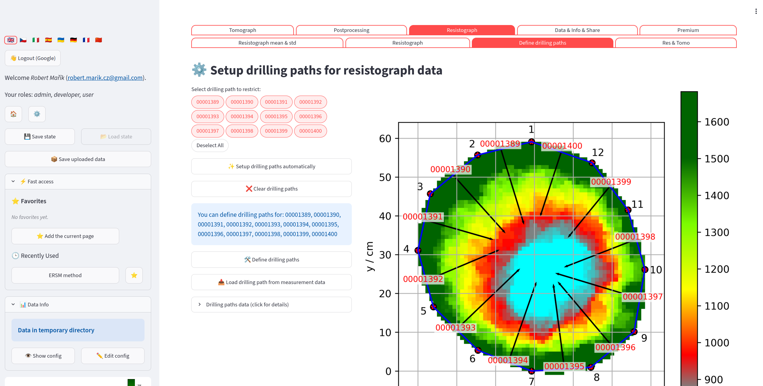
The GUI allows to set the drilling paths for each file. The paths are used to overlay the resistograph data on the tomogram.
Menu: Resistograph → Define drilling paths
Maps each resistograph file to a physical path on the cross-section, so the curves can be overlaid on the tomogram.
Automatic setup: Click “Setup drilling paths automatically” to have the app place each path from the midpoint between adjacent sensor pairs toward the tree center. Review the result on the tomogram preview before proceeding.
Manual setup:
Select the paths you want to define using the pills widget.
Click “Define drilling paths”; the app navigates to the Measurement Tool.
Draw one segment per path.
Return to this page and click “Load drilling path from measurement data” to import the segments you drew.
Click “Clear drilling paths” at any time to reset all paths.
After defining paths, click Save paths to config.yaml to persist them.
Resistograph & Tomogram Overlay
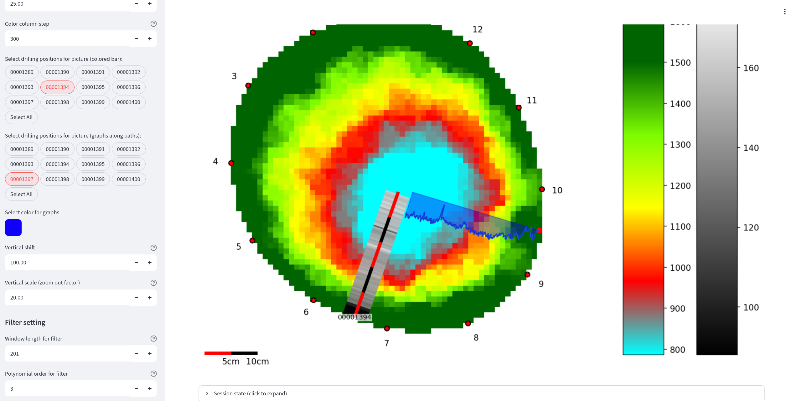
It is possible to merge the data from image reconstruction and data from resistance drilling into a single plot. The resistance drilling data allow two different visualizations: as a line graph or as a colored bar column along the drilling path.
Menu: Resistograph → Res & Tomo
Overlays smoothed resistograph data on the tomogram as colored bar columns along each drilling path.
Sidebar controls:
R_min / R_max — value range for color mapping resistograph readings.
R_depth — how deep along each path to visualize.
R_scale_length — physical length of the scale bar (m).
R_color_column_step — width of each colored bar step.
Color picker for line graphs.
R_vertical_shift / R_vertical_scale — adjust the resistograph graph position alongside the path.
Filter: Savitzky–Golay window and polynomial order for smoothing.
Drill bars selector / Drill graphs selector (pills) — choose which paths appear as colored bars and which as line graphs.
Freeze toggle — freezes all settings to prevent recomputation while you adjust parameters. Unfreeze to apply everything at once.
Click Save to file to write all current settings to the dataset’s config.yaml so they are restored automatically next time.
3D Scans
3D scans of the stem (*.obj with its *.mtl and texture, *.glb, *.gltf) are stored in the scans/ subdirectory of the dataset.
Sensor Position
Menu: Scan tools → Sensor position
Marks the sensors on the 3D scan and derives the sensor geometry and the stem outline from it.
🔍 Detect red markers finds red discs (markers with a pin in the centre) in the scan texture (OBJ with texture). Sensors in the measurement starts from the sensor count of the opened measurement; when fewer discs are found, the gaps are searched again with a looser colour threshold and these points are shown in orange as uncertain. Points can be added, moved or removed by hand.
The sensors are numbered around the stem from Sensor 1, in the direction chosen below the 3D view (anticlockwise or clockwise viewed from above; the default comes from the measurement, see Tomograph files). Number in the order clicked keeps the order of clicking instead.
💾 Save sensor geometry to the dataset writes
scan_geometry.csvto the measurement folder andsensor_geometry.json(3D sensor positions, plane and outline) next to the scan. Existing files are replaced only after ticking the confirmation. When the same scan is opened again, the saved sensors and outline are loaded; a geometry saved for another scan file is ignored. A geometry whose cross-section plane is tilted more than 45° from horizontal is rejected. In a dataset with data sources, the savedscan_geometry.csvis registered as a source (a source already in use is reloaded); choose it on the page Data Sources. Used for Geometry, the scan also gives the stem Boundary (its outline), so the tomogram is reconstructed and drawn with the scan outline. In an older dataset without data sources, choose Geometry: Scan in the sidebar.
Cross Section
Menu: Scan tools → Cross section
Cuts the scan and fits the cross-section polygon. With the three.js viewer, Show tomogram or photo on the cut places an image in the 3D scan (for viewing, not a 3D measurement):
Tomogram — the last computed tomogram (cells, rays or both as on the tomogram page, colours by the Plot function, line width Ray line width). With the sensor geometry saved on the Sensor position page, the tomogram is fitted to the saved 3D sensors without scaling: exactly for a tomogram computed with the scan geometry, as a best fit with the sensor offsets reported for the device geometry. Without a saved geometry, Shift + click Sensor 1 on the scan and click Confirm changes in the viewer; the numbering direction and the Sensor 1 position can be saved to
config.yaml.Photo of the cross section — the photo and tracing from Photo Assessment, fitted through the sensors marked on the photo to the saved scan sensors (rotation, scale, mirroring); the deviations are reported.
Draw the image over the stem (on by default) keeps the whole stem visible with the image seen through it; switched off, the stem above the image is cut away. Drawing the image needs a recent streamlit-3d-viewer; the page says so if the installed version is too old. For a tomogram fitted to saved sensors, the page shows a Reproduce in Jupyter snippet that draws the same view with PyVista (tomotree.scans.scantree.tomogram_on_scan).
Data Sources
Menu: Data & Info & Share → Data sources
The measured data of a dataset — Geometry (sensor positions), Times (travel times or speeds) and Boundary (stem outline) — are imported into config.yaml; each file they come from is a source (tomograph file, CSV table, scan_geometry.csv from Sensor Position). The page lists the files of the dataset:
Use for — choose which quantities are taken from the file. A 3D scan used for Geometry also brings its Boundary; a Boundary can also be chosen alone (e.g. the scan outline with the device geometry).
✅ Apply uses all chosen sources at once; the dataset is reloaded and everything is recomputed. ✖️ Discard forgets the choices.
📥 Import registers a new file, 🔄 Reload reads a changed file again. Data edited by hand in the config editor are reported; ✏️ Keep the edited … marks them as edited (
manual), ↩️ Restore … from the file brings back the file data.
A scan geometry needs travel times (not only speeds) as the source of Times. Settings numbered by sensors (disabled rays, bark thickness per node, …) stay with the geometry they belong to. The format is described in the configuration file.