Quick Start Guide
This guide is intended for users who want to quickly get TomoTree up and running in Jupyter notebook. For installation see the Installation Guide.
Loading a measurement
In Jupyter you do not need the config.yaml of the web application. Load the measurement
from the tomograph file or from CSV tables and pass it to tomotree.analysis.reconstruct
as a dict with nodes (sensor coordinates in m) and speeds (m/s) or times (s):
import pandas as pd
from tomotree import analysis
from tomotree.dataset import read_device_file

data = read_device_file("jicin_08.f3d")        # Fakopp .f3d, PiCUS .pit or Arbotom .abt
# data = {"nodes": pd.read_csv("demo/data/tree08_sensors.csv", index_col="sensor"),
#         "times": pd.read_csv("demo/data/tree08_times.csv", index_col="sensor")}
t = analysis.reconstruct(data, method="ERSM", nx=41, ny=41)
t.plot()
read_device_file(path, layer=None) reads the sensor positions and travel times the same
way as the web application opens a folder with only that file; layer selects a layer of a
multi-layer measurement (default: the first one). The CSV files in demo/data/ (described in
demo/data/README.md) were exported this way. More examples are in demo/demo_01_*.py …
demo_09_*.py.
missing_inputs(data, directory, requires) lists what a dataset lacks before you compute;
the web application runs the same check before it opens a page:
from tomotree.dataset import load_dataset, missing_inputs

config, data = load_dataset("Jičín_05")
missing_inputs(data, "Jičín_05", ["geometry", "measurements", "resistograph"])   # [] = complete
Basic usage
Initialize tomogram with sensor positions and velocity data
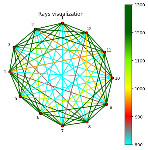
This cell sets up the basic tomogram object with 12 sensors and their measured ultrasound velocities. The symmetric parameter ensures we work with averaged ray paths in both directions.
# Import required libraries and functions
import tomotree as tomo  # Main TomoTree package for tomographic reconstruction
import numpy as np  # Numerical computations
import matplotlib.pyplot as plt  # Plotting graphs
from tomotree.util import show_grid  # Helper function for displaying the grid

# Define sensor positions (node coordinates) - 12 sensors
# Format: [x1, y1, x2, y2, ..., x12, y12]
# Each row represents one sensor with coordinates (x, y)
nodes = np.array([
        0.000000000000000000e+00,0.000000000000000000e+00,
        -1.423512143280224185e-01,-3.243658088235288478e-02,
        -2.547529511272511593e-01,-1.277729779411764799e-01,
        -2.779073009818450735e-01,-2.576985294117646874e-01,
        -2.225714384149889424e-01,-3.876479779411763915e-01,
        -1.155980768557571953e-01,-4.782270220588235032e-01,
        0.000000000000000000e+00,-5.440000000000000391e-01,
        1.314503633637385815e-01,-5.237564338235293215e-01,
        2.339414392116714869e-01,-4.305477941176470424e-01,
        2.650568812590387568e-01,-2.901617647058822858e-01,
        2.237194098650501228e-01,-1.547049632352941462e-01,
        1.294254175011995411e-01,-5.069577205882350862e-02,
        ]).reshape(-1,2)  # Reshape to 12x2 matrix (12 sensors, 2 coordinates)

# Matrix of ultrasound velocities between sensors (m/s) - 12x12 matrix
# np.nan on diagonal (no signal from one sensor to itself)
speeds = np.array([
        np.nan,1678,1501,1336,1146,793,637,738,972,1203,1400,1503,
        1678,np.nan,1546,1439,1329,1075,600,579,807,953,1300,1465,
        1501,1546,np.nan,1517,1528,1280,989,859,693,764,1135,1314,
        1336,1439,1517,np.nan,1592,1402,1246,1179,865,674,961,1142,
        1146,1329,1528,1592,np.nan,1377,1291,1280,1064,756,644,817,
        793,1075,1280,1402,1377,np.nan,1263,1402,1256,1040,711,567,
        637,600,989,1246,1291,1263,np.nan,1859,1545,1355,1095,857,
        738,579,859,1179,1280,1402,1859,np.nan,1474,1431,1215,989,
        972,807,693,865,1064,1256,1545,1474,np.nan,1563,1355,1249,
        1203,953,764,674,756,1040,1355,1431,1563,np.nan,1288,1320,
        1400,1300,1135,961,644,711,1095,1215,1355,1288,np.nan,1513,
        1503,1465,1314,1142,817,567,857,989,1249,1320,1513,np.nan,
        ]).reshape(12,12)  # Reshape to 12x12 matrix (12 sensors x 12 sensors)

# Set the size of the reconstructed grid
NX, NY = 100, 100  # 100x100 grid for the tomographic map

# Create tomogram object
# - nodes: sensor positions
# - speeds: measured ultrasound velocities
# - nx, ny: resolution of the output grid
# - symmetric=True: assume symmetric measurements (averaging both propagation directions)
tomogram = tomo.Tomo(nodes, speeds, nx=NX, ny=NY, symmetric=True)
# Plot the rays in the initial tomogram before reconstruction
tomogram.plot(rays=True, grid=False, speed_max=1300, speed_min=800)

# Get current matplotlib axis and set title
ax = plt.gca()
ax.set_title('Rays visualization')
plt.show()
Perform ERSM reconstruction and estimate sound wood speed
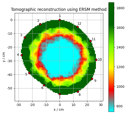
This cell executes the tomographic reconstruction algorithm (ERSM method), optimizes the result, and estimates the reference speed in healthy wood. The output shows the reconstructed tomographic map with color-coded velocity values.
# Perform tomographic reconstruction using ERSM method
tomogram.do_ERSM_method()

# Optimize the tomogram - rescale speed values to match
# measured data as closely as possible
tomogram.optimize_back_tomogram()

# Estimate sound velocity in undamaged (healthy) part of wood
# Used as reference value for interpreting results
# Faster sound = healthy wood; slower sound = damaged/hollow part
sound_wood_speed = tomogram.estimate_sound_wood_speed()

# Plot the resulting tomographic map
# rays=False: don't show sound rays
# grid=True: display the grid
# speed_max: maximum on color scale (healthy wood)
# speed_min: minimum on color scale (40% of healthy - damaged part)
tomogram.plot(rays=False, grid=True, speed_max=sound_wood_speed,
speed_min=(sound_wood_speed)*0.4)  # Range: 40% to 100% of healthy wood

# Get current matplotlib axis and set title
ax = plt.gca()
ax.set_title('Tomographic reconstruction using ERSM method')

# Display grid on the map
show_grid(ax)

# Show the created plot
plt.show()
Wall thickness measurement
Measure wall thickness between sensor pairs
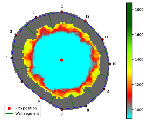
This cell analyzes the tomogram to determine the thickness of healthy wood between each pair of sensors, useful for detecting cavities, decay, and damage in the material.
# Import function for measuring wall thickness and detecting hollow areas
from tomotree.util import measure_walls

# Measure thickness of undamaged part between sensors
# Parameters:
# - tomogram: processed tomogram from previous step
# - sound_wood_speed: speed_max, sound velocity in healthy wood (reference value)
# - sound_wood_speed*0.5: speed_min; the threshold between sound and damaged wood
#   defaults to the mean of speed_max and speed_min (75% of sound wood speed here)
# - plot_figure=True: creates visual representation of measurements
result = measure_walls(tomogram, sound_wood_speed, sound_wood_speed*0.5, plot_figure=True)

# Display results in table
# Sensor1: first sensor in the pair
# Sensor2: second sensor in the pair
# Wall_thickness: measured thickness of healthy wood part between sensors
result['df'][['Sensor1','Sensor2','Wall_thickness']]
| Sensor1 | Sensor2 | Wall_thickness | |
|---|---|---|---|
| 0 | 1 | 2 | 0.087950 |
| 1 | 2 | 3 | 0.091520 |
| 2 | 3 | 4 | 0.068051 |
| 3 | 4 | 5 | 0.079620 |
| 4 | 5 | 6 | 0.052659 |
| 5 | 6 | 7 | 0.046520 |
| 6 | 7 | 8 | 0.080642 |
| 7 | 8 | 9 | 0.086946 |
| 8 | 9 | 10 | 0.048272 |
| 9 | 10 | 11 | 0.046359 |
| 10 | 11 | 12 | 0.046236 |
| 11 | 12 | 1 | 0.053496 |