Open source software for acoustic tomography of trees.
Five reconstruction methods, detection of cracks, 3D scans of the stem, resistograph.
Reads Fakopp (.f3d), PiCUS (.pit) and Arbotom (.abt) measurements as well as CSV files.
Graphical user interface in the web browser, in seven languages, no programming needed.
The same computations as a Python library for Jupyter notebooks.
Available online, as a Python package or as a Docker container.
Five reconstruction methods
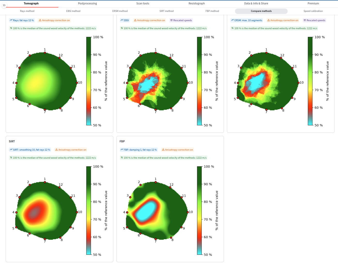
Rays (thin or fat rays), EBSI, ERSM, regularized SIRT with fat rays and
filtered back projection (FBP).
The page Compare methods shows the tomograms of all methods side by side with the same
settings and a common colour scale, with a table of the misfit of the measured times.
Anisotropy correction, bark thickness, rescaling of speeds and the correction by back projection.
No black box: each method is documented, the settings of every tomogram are shown in badges above it.
Changed settings do not recompute at once: the previous tomogram stays faded with the list of
changes until you press Recompute tomogram.
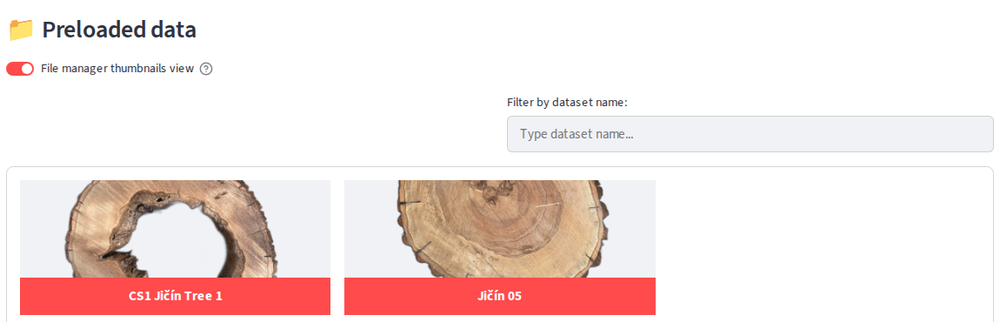
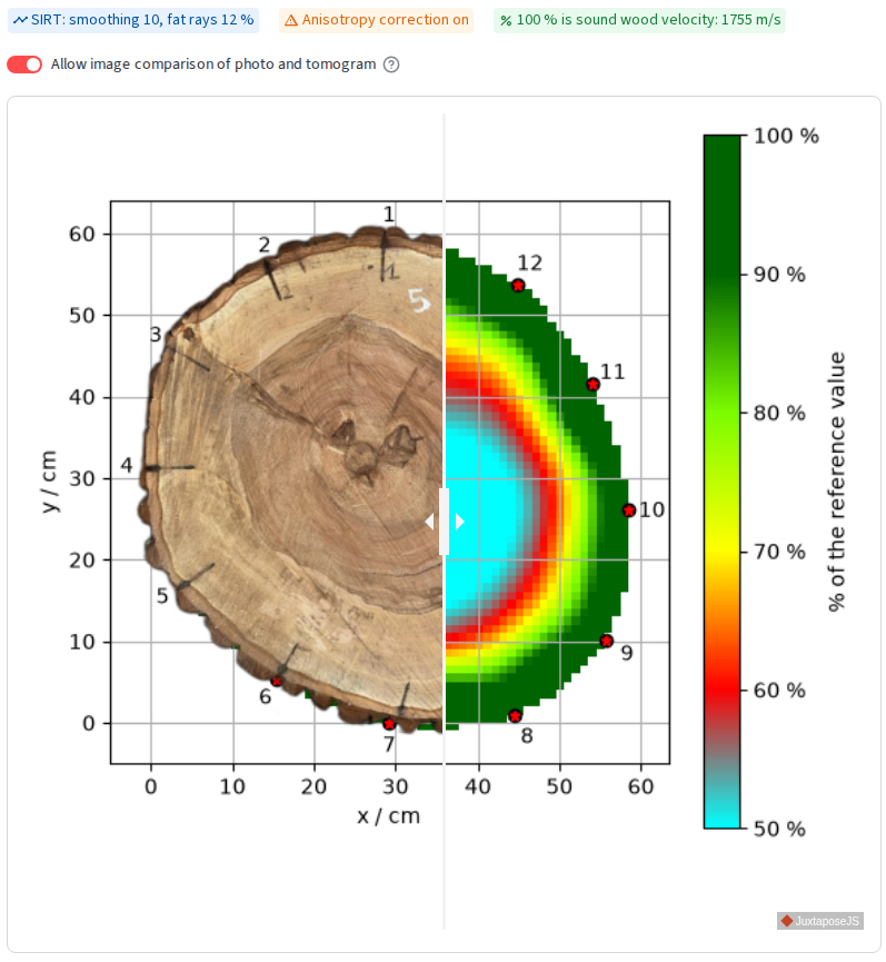
Tomogram and the photo
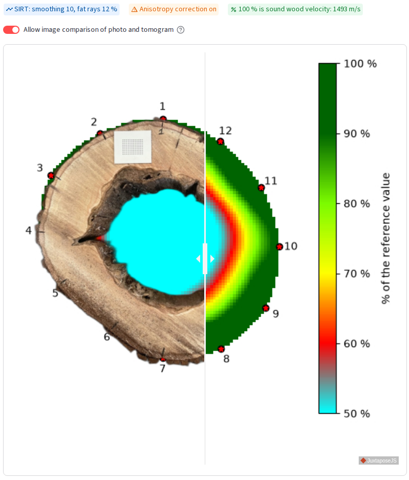
The tomogram can be compared with the photo of the actual cross section by a slider.
The default colour scale is the percentage of the sound wood velocity, so a sound tree
stays green; percentile and absolute scales are also available.
Static or interactive plots (plotly, bokeh), custom colormaps, statistics of the tomogram.
Acoustic rays
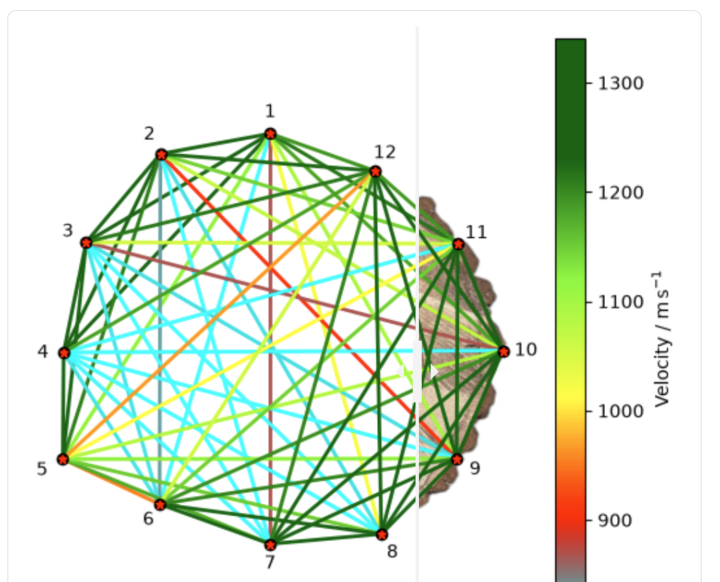
Visualization of the acoustic rays in the cross section, alone or over the photo.
Speed filter for rays allows to focus on the slowest or the fastest rays.
The Select rays dialog disables single rays by clicking and suggests suspicious rays:
rays leaving the stem outline and pairs whose two directions disagree.
Angle plots show the ray speed as a function of the declination from the radial direction.
Cracks: dividing line
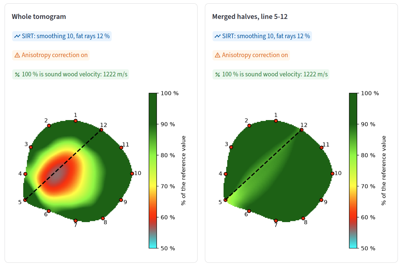
Linear defects such as cracks look like cavities in the tomogram. TomoTree can tell them apart.
The cross section is split by a chord between two sensors, each half is reconstructed from
the sensors on its side and the halves are merged.
A defect along the line disappears in the merged tomogram, a cavity stays.
Metrics (delay of the rays crossing the line, change of the defect area) and an automatic
search for the dividing line of a crack.
3D scans of the stem
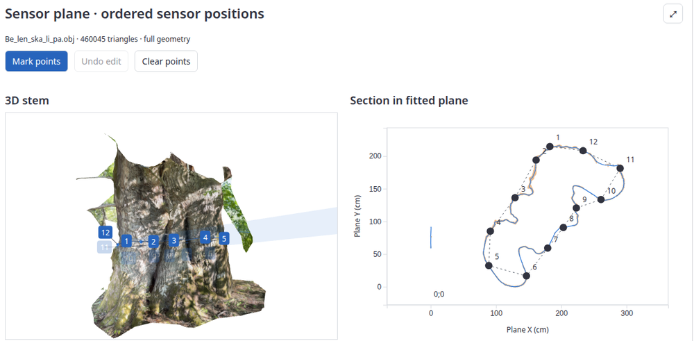
Load a 3D scan of the stem (OBJ, GLB) made e.g. by a phone app.
Red sensor markers are detected automatically and numbered around the stem; points can be
added or moved by hand.
The sensor plane is fitted, the stem outline is cut from the scan and the sensor geometry is
saved to the dataset.
The scan outline becomes the boundary of the tomogram; the tomogram or the photo can be shown on the cut.
Cross section tools compute the area and the mechanical characteristics of the scanned cross section.
Speed calibration
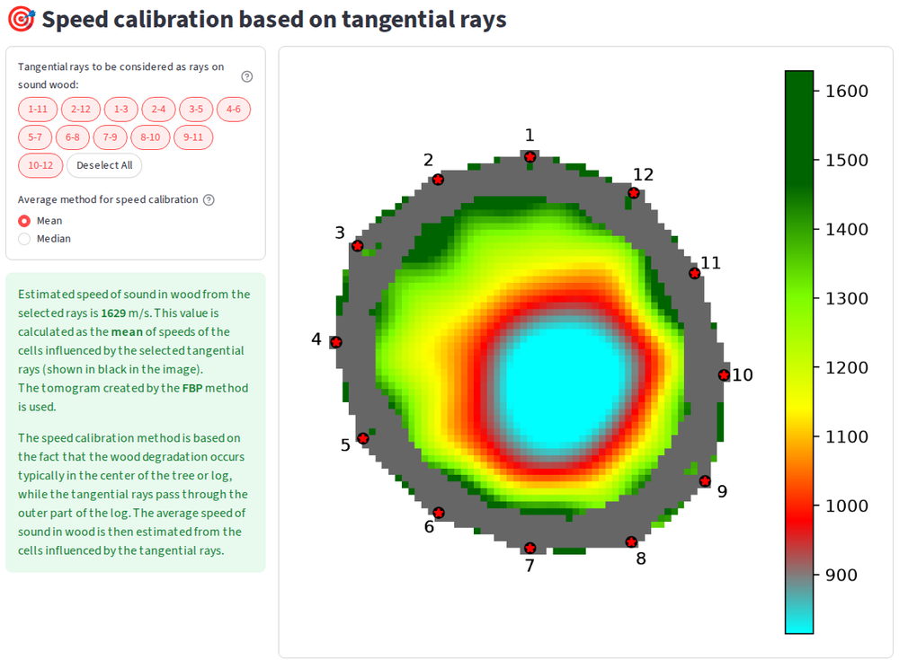
Speed calibration sets the sound speed in the sound wood. It is the reference for tomogram interpretation.
The sound speed is estimated from the cells influenced by the tangential rays.
The user can finetune the sound speed by excluding the rays close to the defect.
Binary tomogram
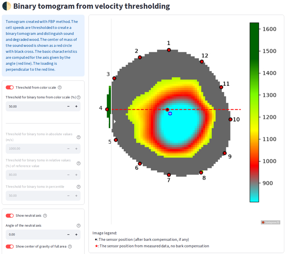
Binary tomogram separates the sound wood from the degraded wood or the cavities.
The threshold can be set interactively and the effect on the binary tomogram is shown immediately.
The area of the sound wood, the wall thicknesses and the center of gravity are computed.
Given a neutral axis, the physical characteristics important for tree stability are estimated.
Photo assessment
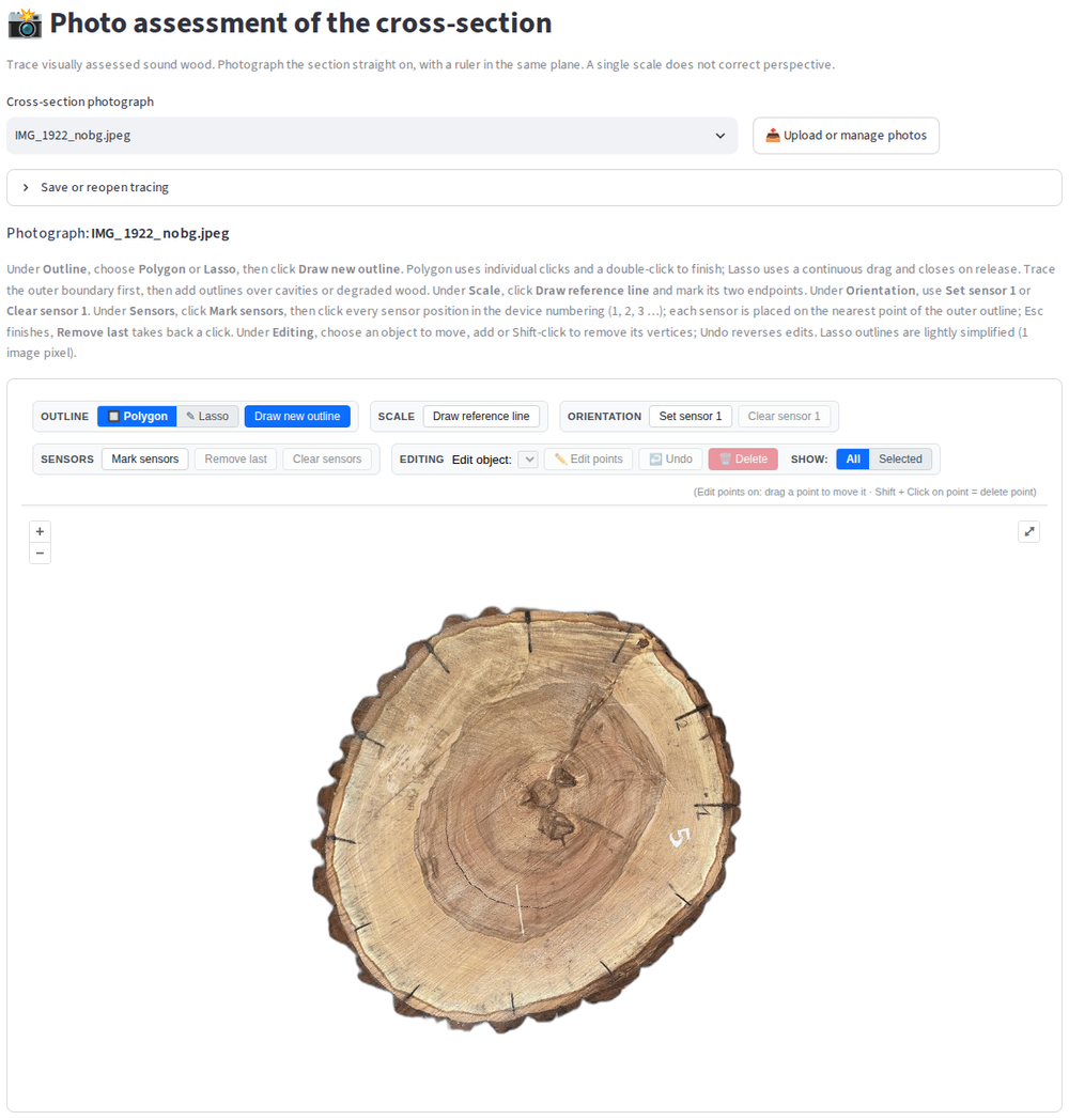
Trace the sound wood, cavities and decay in the photo of the cross section (polygon or lasso).
Set the scale by a reference line and mark the sensors on the photo.
Areas and wall thicknesses from the photo can be compared with those from the tomogram.
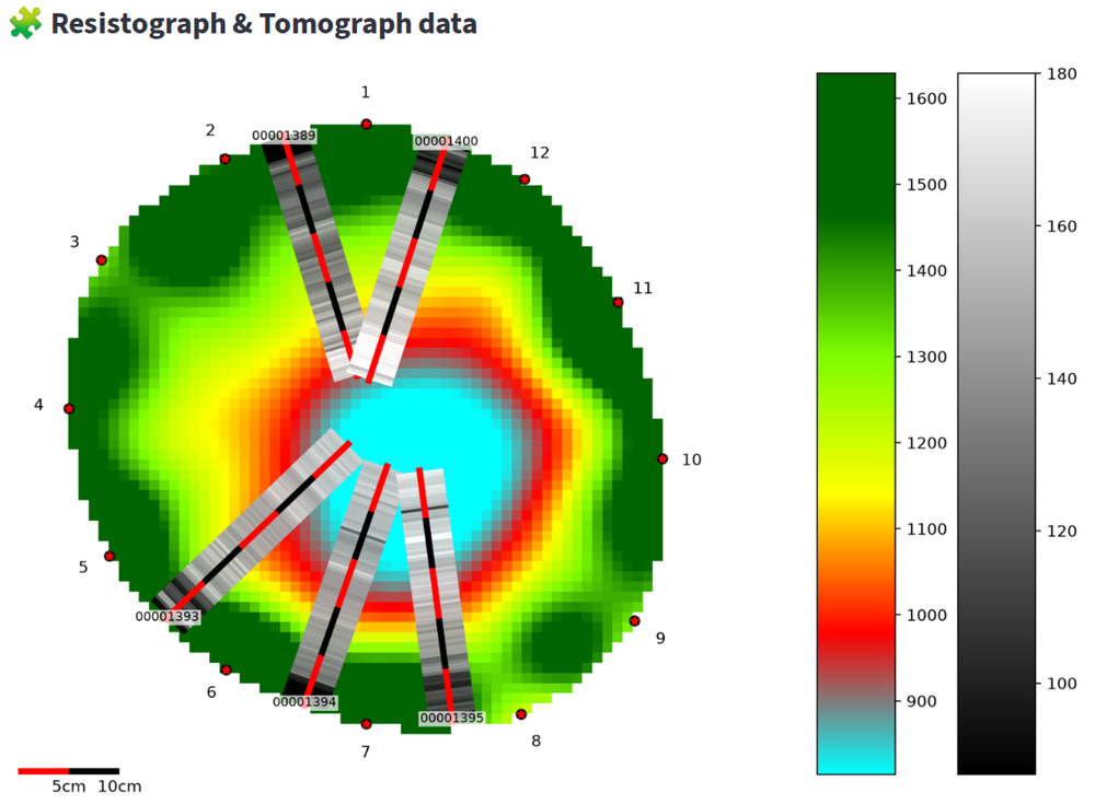
Resistograph
Visualization of resistograph curves, their mean and standard deviation.
Drilling paths are defined on the tomogram.
Combined plots draw the resistograph profiles directly over the tomogram.
Data sources
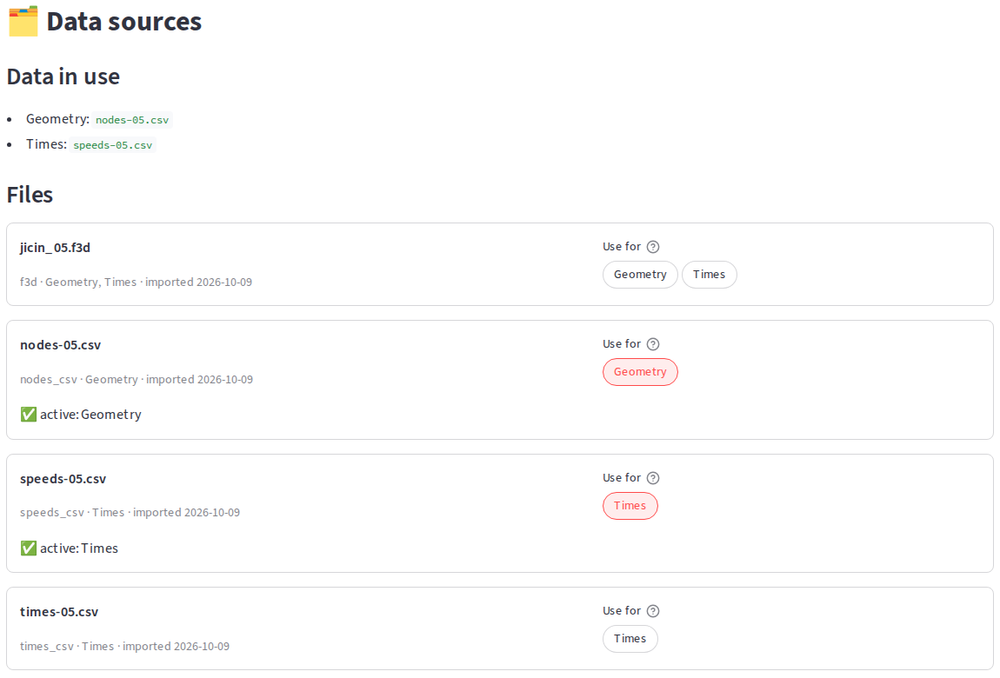
Measured data enter a dataset by an explicit import; every file is recorded with its date and checksum.
The page Data sources shows the files and lets you choose the geometry and the times in use,
e.g. the sensor geometry from a 3D scan and the times from the tomograph file.
Changed or new files are detected and imported again.
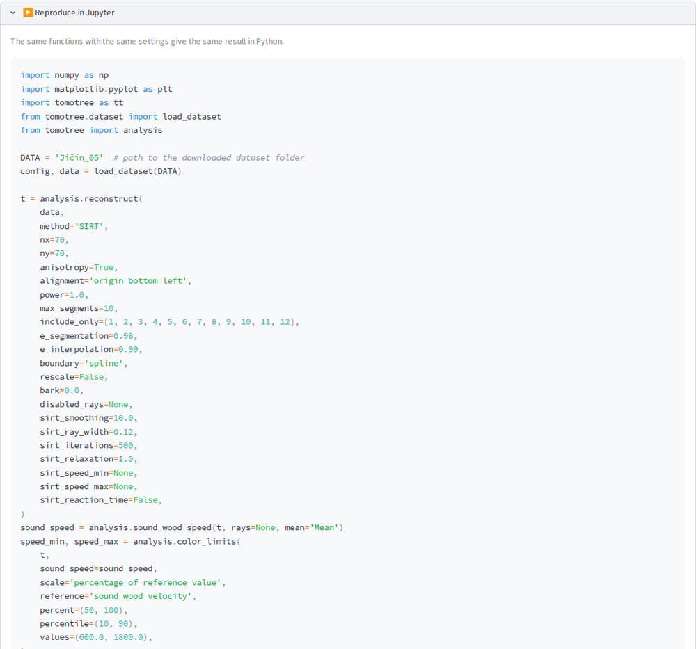
Reproduce in Jupyter
Every analysis page shows a Python snippet which gives the same result in Jupyter.
The snippet uses the same library functions with the same settings as the GUI.
Use the GUI to explore the data and the library for batch processing or publications.
Getting started
The stable GUI contains well tested code which allows to utilize TomoTree without programming skills.
The development version of the GUI contains new features which will be propagated to the stable branch after testing period.
You can also run TomoTree locally using Docker or Conda. See the documentation on GitHub.
The development of TomoTree is supported by the Ministry of Education, Youth and Sports
of the Czech Republic, project ERC CZ no. LL1909 “Tree Dynamics: Understanding of Mechanical
Response to Loading (DYNATREE)” and MSCA FELLOWSHIP CZ MENDELU CZ.02.01.01/00/22_010/0008893
“Wood Degradation in the Urban Environment (WooDU)”.
Access to CESNET storage facilities provided by the project “e-INFRA CZ” under the programme “Projects of Large Research, Development, and Innovations Infrastructures” LM2023054), is greatly appreciated.